Inelastic Collisions

INELASTIC COLLISIONS

Purpose:

     To analyze the motion of two low friction carts during an inelastic collision and verify that the law of
conservation of linear momentum is obeyed.

Equipment:

     Computer with Logger Pro software, lab pro, motion detector, horizontal track, two carts, 500 g
masses(3), triple beam balance, bubble level

Introduction:

     This experiment uses the carts and track as shown in the figure.  If we regard the system of the two
carts as an isolated system, the momentum of this system will be conserved.  If the two carts have
a perfectly inelastic collision, that is, stick together after the collision, the law of conservation of
momentum says

Pi = Pf

m1v1 + m2v2  =  (m1 + m2)V

where v1 and v2 are the velocities before the collision and V is the velocity of the combined mass 

after the collision.

Procedure:

1.   Set up the apparatus as shown in Figure 1.  Use the bubble level to verify that the track is as
level as possible. Record the mass of each cart.  Connect the lab pro to the computer and the
motion detector to the lab pro. On the computer, start the Logger Pro software, open the
Mechanics folder and the Graphlab file.

2.   First, check to see that the motion detector is working properly by clicking the Collect button to
start collecting data.  Move the cart nearest the detector back and forth a few times while
observing the position vs time graph being drawn by the computer.  Does it provide a
reasonable graph of the motion of the cart?  Remember to be aware of unwanted reflections
caused by objects in between the motion detector and the cart.  Also, position the carts so that
their velcro pads are facing each other.  This will insure that they will stick together after the
collision.

3.   With the second cart (m2) at rest give the first cart (m1) a moderate push away from the motion
detector and towards m2.  Observe the position vs time graph before and after the collision.
What should these graphs look like?  Draw an example:
The slope of the position vs. time graph directly before and directly after the collision give the
velocity directly before and directly after the collision.  To avoid the problem of dealing with
friction forces (Remember, we are assuming the system is isolated.), we will find the velocity of
the carts at the instant before and after the collision.
Is this a good approximation? Why or why not?
For the velocity before the collision, select a very small range of data points just before the
collision.  Avoid the portion of the curve which represents the collision.  Choose
Analyze/Linear Fit.  Record the slope (velocity) of this line.  Repeat for a very small range of
data points just after the collision.  Record this slope (velocity) as well.

4.   Repeat for two more collisions.  Calculate the momentum of the system the instant before and
after the collision for each trial and find the percent difference.  Put your results in an Excel data
table. Show sample calculations here:

5.   Place an extra 500 g on the second cart and repeat steps 3 and 4.  Sketch one representative
graph showing the position vs time for a typical collision. (What do velocity vs. time and
acceleration vs. time look like?6. Remove the 500 g from the second cart and place it on the first cart.  Repeat steps 3 and 4.

7.   Find the average of all of the percent differences found above.  This average represents your
verification of the law of conservation of linear momentum.  How well is the law obeyed based
on the results of your experiment? Explain.

8.   For each of the nine trials above calculate the kinetic energy of the system before and after the
collision.  Find the percent kinetic energy lost during each collision.  Put this information in a
separate data table.  Show sample calculations here:

9.   Do a theoretical calculation for ΔK/K in a perfectly inelastic collision for the three situations:

1. a mass, m, colliding with an identical mass, m, initially at rest.
2. a mass, 2m, colliding with a mass, m, initially at rest.
3. a mass, m, colliding with a mass, 2m, initially at rest.

Balanced Torques and Center of Gravity

Balanced Torques and Center of Gravity

Objective:  

     To investigate the conditions for rotational equilibrium of a rigid bar and to determine the center of gravity of a system of masses.

Materials: 

• 1 Meter Stick
• 3 Meter Stick clamps (knife edge clamp)
• 1 Balance Support
• 1 Mass Set of Various Masses 
• 3 Weight hangers
• 1 Unknown Masse
• 1 Balance                                             

Procedure:

1. Balance the meter stick in the knife edge clamp and record the position of the balance point.

2. Select two different masses (100 grams or more each) and using the meter stick clamps and weight hangers, suspend one on each side of the meter stick support at different distances from the support. Adjust the positions so the system is balanced. Record the masses and positions. Sum the torques about your pivot point O and compare with the expected value.

3. Place the same two masses used above at different locations on the same side of the support and balance the system with a third mass on the opposite side. Record all three masses and positions. Calculate the net torque on this system about the point support and compare with the expected value.

4. Replace one of the above masses with an unknown mass. Readjust the positions of the masses until equilibrium is achieved, recording all values. Using the equilibrium condition for rotational motion, calculate the unknown mass. Measure the mass of the unknown on a balance and compare the two masses by finding the percent difference.

5. Place about 200 grams at 90 cm on the meter stick and balance the system by changing the balance point of the meter stick. From this information, calculate the mass of the meter stick. Compare this with the meter stick mass obtained from the balance.

6. With the 200 grams still at the 90 cm mark, imagine that you now position an additional 100 grams mass at the 30 cm mark on the meter stick. Calculate the position of the center of gravity of this combination (two masses and meter stick). Check your result by actually placing the 100 g at the 30 cm mark and balancing this system. Compare the calculated and experimental results.

Human Power

Human Power

Purpose: 

     To determine the power output of a person.

Equipment: 

• 2 Two-meter Meter Sticks
• 1 Stopwatch
• 1 Kilogram-bathroom Scale 
• Humans

Introduction: 

     Power is defined to be the rate at which work is done or equivalently, the rate at which 

energy is converted from one form to another.  In this experiment you will do some work 

by climbing from the first floor of the science building to the second floor.  By measuring  

the vertical height climbed and knowing your mass, the change in your gravitational  

potential energy can be found: 

∆ PE = mgh 

Where m is the mass, g the acceleration of gravity, and h is the vertical height gained.  

Your power output can be determined by  

Power  = 

∆ PE  , 

∆t

where ∆t is the time to climb the vertical height h. 

                             

Procedure: (from lab handout)

1.   Determine your mass by weighing on the kilogram bathroom scale.  Record your mass in kg.. 

2.   Measure the vertical distance between the ground floor and the second floor for the science 

building.  This can most easily be done by using two meter long metersticks held end to end in the 

stairwell at the west end of the building.  Make a careful sketch of the stairwell area that explains 

the method used to determine this height. 

3.   Designate a record keeper and a timer for the class. At the command of the timing person, run or 

walk (whatever you feel comfortable doing) up the stairs from the ground floor to the second 

floor.  Be sure that your name and time are recorded by the record keeper.  

4.   After everyone in the class has completed one trip up the stairs, repeat for one more trial.  

5.   Return to class and calculate your personal power output in watts using the data collected from

each of your climbing trip up the stairs.  Obtain the average power output from the two trials. 

'

6.   Put your average power on the board and then calculate the average power for the entire class once 

everyone has reported their numbers on the board.

7.   Determine your average power output in units of horsepower. 

Centripetal Force

Centripetal Force

Purpose:      
     
     To verify Newton's second law of motion for the case of uniform circular motion.

Equipment: 

• 1 Centripetal Force Apparatus
• 1 Metric Scale
• 1 Vernier Caliper
• 1 Stop Watch
• 1 Slotted Weight Scale
• 1 Weight Hanger
• 1 Triple Beam Balance

Introduction: 

     The centripetal force apparatus is designed to rotate a known mass through a circular path of known radius. By timing the motion for a definite number of revolutions and knowing the total distance that the mass has traveled, the velocity can be calculated. Thus, the centripetal force, F, necessary to cause the mass to follow its circular path can be determined from Newton's second law: 

F= (mv^2)/r

Where m is the mass, v is the velocity, and r is the radius of the circular path. Here we have used the fact that for uniform circular motion, the acceleration, a, is given by the formula:

a= (v^2)/r

Procedure:   (from lab handout)

1.      For each trial the position of the horizontal cross-arm and the vertical indicator 

post must be such that the mass hangs freely over the post when the spring is 

detached. After making this adjustment, connect the spring to the mass and 

practice aligning the bottom of the hanging mass with the indicator post while 

rotating the assembly. 

2.     Measure the time for 50 revolutions of the apparatus. Keep the velocity as 

constant as possible by keeping the pointer on the bottom of the mass aligned with 

the indicator post. A white sheet of paper placed as a background behind the 

apparatus can be helpful in getting the alignment as close as possible. Using the 

same mass and radius, measure the time for three different trials. Record all data 

in a neat excel table (see 6). 

3.     Using the average time obtained above, calculate the velocity of the mass. From 

this calculate the centripetal force exerted on the mass during its motion. 

4.     Independently determine the centripetal force by attaching a hanging weight to 

the mass until it once again is positioned over the indicator post (this time at rest). 

Since the spring is being stretched by the same amount as when the apparatus was 

rotating, the force stretching the spring should be the same in each case.  

a.   Calculate this force and compare with the centripetal force obtained 

in part 3 by finding the percent difference.   

b.   Draw a force diagram for the hanging weight and draw a force 

diagram for the spring attached to the hanging mass: 

5.      Add 100 g to the mass and repeat steps 2, 3 and 4 above. 

6.      The following data should be calculated and recorded in your excel table: 

a.   Mass and radius for each trial. 

b.   Average number of revolutions/sec (frequency) for each trial. 

c.   Linear speed for each trial. 

d.   Calculated and measured centripetal force for each trial and their percent 

difference.

Setup:

Pictures of Lab Equipment and Demonstrations

Hanging Bob Aligned with Marking Rod

Keeping a Rhythm while I spin the Centripetal Force Apparatus

Measuring Expected Radius and Tension by Hanging mass off of Pulley

 Data:

Force Diagram for the Hanging Weight

     mass = 446.1 g = .4461 kg

radius = 16.6 cm = .166 m

frequency = 50/s

F = (m*v^2)/r

Conclusion:

     In this lab I learned how to measure centripetal force and how to properly use a vernier caliper.  According to our table of data and results, we can say that when the radius is kept constant and the mass increases, the centripetal force increases. Our average calculated centripetal force when added the 100 g is very close to the measured centripetal force. The last one (added 50 g) is much closer than the first one.  We can say that our results are accurate and convincing. In this lab, we verify Newton's second law of motion  (uniform circular motion). The acceleration (a) of the object is directly proportional to the net force, and is inversely proportional to the mass (m). F= ma. In this particular case, the direction of net force points to the center of the circle, where a=v^2/r.  Possible sources of error in this lab were when I was spinning the mass on the string, I didn't always spin it with a constant velocity, the person timing the fifty revolutions might not have stopped the stopwatch exactly when the mass made its fiftieth revolution, and the string and spring have mass as well, but we do not really compare to the weight we had attached so we could say we neglected those masses.  To improve the lab, we could maybe use something like a Doppler Radar or something to precisely measure the time it takes for one revolution and would therefore decrease human error by a substantial amount.

Drag Force on Coffee Filters

Drag Force on Coffee Filters

Purpose: To study the relationship between air drag forces and the velocity of a falling object.

Equipment:

• 1 Computer with Logger Pro software
• 1 Lab pro
• 1 Motion detector
• 9 Coffee filters
• 1 Meter stick.

Introduction: 

     When an object moves through a fluid, such as air, it experiences a drag force that opposes its motion. This force generally increases with velocity of the object. In this lab, we are going to investigate the velocity dependence of the drag force. We start by assuming the drag force, FD, has a simple power law dependence on the speed given by the formula:

FD= K*(v)^n

(where the n-th power is going to be determined by our experiment)

     In this lab, we will investigate drag forces acting on a falling coffee filter. Because of the large surface area and low mass of these filters, they will reach terminal speed soon after being released.

Procedure: (from lab handout)

     You will be given a packet of nine nested coffee filters. It is important that the shape of this packet stays the same throughout the experiment so do not take filters apart or otherwise alter the shape of the packet. Why is it important for the shape to stay the same?

It is important to maintain the shape of the packet because drag force is proportional to the 1/4 cross-section area of the object. If we change the shape of the object (packet of coffee filters), we would change the cross-section area giving us an inaccurate result for drag force. We would not keep consistency.

1. Login to your computer . Start the Logger Pro software, open the Mechanics folder and the Graphlab file. Do not forget to label the axes of the graph and create an appropriate title for the graph. We set the data collection rate to 30 Hz.
2. We place the motion detector on the floor facing upward (move any objects around it because may cause reflection) and hold the packet of nine filters at a minimum height of 1.5 m directly above the motion detector. Use the meter stick to measure that distance from motion detector to coffee filters. Start the computer collecting data, and then release the packet. What shoud the position vs time graph look like? Explain
   

   The curve decreases pretty fast at first. Then, at some point, the curve turns to be linear (constant slope).
3. Verify that the data are consistent. If not, repeat the trial. Examine the graph and using the mouse, select (click and drag) a small range of data points near the end of the motion where the packet moved with constant speed. Exclude any early or late points where the motion is not uniform.
4. Use the curve fitting option from the analysis menu to fit a linear curve (y=mx+b) to the selected data. Record the slope (m) of the curve from this fit. What should this slope represent?              The slope of this graph will represent the terminal speed of the object. Slope of position vs time graph is equal to the velocity of the object. In this case, terminal speed.
5. Repeat this measurement at least 4 more times, and calculate the average velocity. Record all data in an excel data table.
6. Carefully, remove one filter from the packet and repeat the procedure in parts 2,3,4,5 for the remaining packet of 8 filters. Keep removing filters one at a time and repeating the above steps until you finish with a single coffee filter. Print a copy of one of your best x vs t graphs that show the motion and the linear curve fit to the data for everyone in our group (Graph only).
7. In Graphical Analysis, create a two column data table with packet weight (number of filters) in one column and average terminal speed ([v]) in the other. Make a plot of packet weight (y-axis) vs terminal speed not velocity (x-axis). Choose appropriate labels and scales for the axes of your graph. Be sure to remove the "connecting lines" from the plot. Perform a Power law fit and record the power, n, given by the computer. Obtain a printout. Check the % error between your experimentally determined n and the theoretical value before you make a printout. 
8. Since the drag force is equal to the packet weight, we have found that dependence of drag force on speed. Write equation 1 above with the value of n obtained from your experiment. Put a box around this equation. Look in the section on drag forces in your text and write down the equation given there for the drag force on an object moving through a fluid. How does your value of n compare with the value given in the text? What does the other fit parameter represent? Explain. 
   
   
   Data and Results:
   
   
   Graph from one of our trials:

   

   Position vs. Time Graph
   slope = 2.420 m/s; terminal speed = 2.420 m/s

   
        
   
   
        We must use the Power Law Fit in order to find the best fitting curve for our graph. The equation is Y= 1.48X^(2.17) where X is equal to terminal speed and Y is equal to the number of coffee filters. We find n to be equal to 2.17. We then had to compare this value of n to the actual value of n given in our book. Actual value of n=2. Our value of n ended up being very close to the actual value of n. The equation given by our book is FD= 1/4Av^n, where n = 2.
   
   

   

   Number of Filters vs. Terminal Velocity Graph
   w/ Power Law Fit Curve

   
   
   Question:  How does the value of n compare with the value given in the textbook? What does the other fit parameter represent?
        We find that n = 2.17 from our power curve fit. This value is almost identical to the actual value of n (n = 2) given to us by our textbook . FD=1/4Av^2 where FD is a force (in this case, mass*acceleration due to gravity), so FD=mg=1/4Av^2; we also found that Y= 1.48X^2.17 (X=terminal speed, Y=number of coffee filters). So, Y*mg= 1/4AX^2 (m = the mass of each coffee filter).
   Conclusion:

        In this lab, we study the relationship between air drag forces and the velocity of a falling object. We can draw some conclusions from our graph and data related to drag force and velocity. When an object starts falling down, its velocity increases. However, there is certain point where its velocity will be constant. At this point, velocity is equal to drag force. We call this velocity terminal velocity. In our graph, we would expect some portion of it to be parabolic shaped and another portion to be linear (where velocity is constant). We know from our equation FD= 1/4Av^2 that as velocity increases, drag force increases as well. As drag increases, acceleration decreases. Some causes of error may be that as the coffee filters fell down, their shapes are easily able to be changed, and since drag force is related to the cross-section area of the object, if shape changes, the drag force will change as well; rounding values is also one source of error that most certainly affected us; and the number of filters vs. the average speed, because since the coffee filters are so light, that they might have been affected by wind, which would cause some unwanted horizontal velocity.

Working with Spreadsheets

Purpose:

To get familiar with electronic spreadsheets by using them in some simple applications.

Equipment:

• 1 Computer with Microsoft EXCEL software.

Procedure: (from lab handout)

1. Your instructor will give you a brief explanation of how a spreadsheet works and show you some 

of the basic operations and functions. 

2. Turn on the computer and load Excel software by clicking on Start, move the mouse over              

Programs them move the mouse over Microsoft Excel and then press the left button. 

3. Create a simple spreadsheet that calculates the values of the following function: 

    f(x) = A sin(Bx + C) 

   

Initially choose values for  of  A = 5, B = 3 and  C = π/3.  Place these values at the right side of the 

spreadsheet in the region reserved for constants.  Put the words amplitude, frequency, and phase 

next to each as an explanation for the meaning of each constant.  Place column headings for "x" 

and "f(x)" near the middle of the spreadsheet, enter a zero in the cell below "x", and enter the 

formula shown above in the cell below "f(x)".  Be sure to put an equal sign in front of the formula.  

Create a column for values of x that run from zero to 10 radians in steps of  0.1 radians.  Use the 

copy feature to create these x values (Don't enter them all by hand!).  Similarly, create in the next 

column the corresponding values of  f(x) by copying the formula shown above down through the 

same number of rows (100 in all). 

4. Once the generated data looks reasonable, copy this data onto the clipboard  by highlighting the 

contents of the two columns and choosing  EDIT/COPY from the menu bar. Print out a copy of 

your spreadsheet (first 20 rows or so) and also print out the spreadsheet formulas (try CTRL~).  Be 

sure that your rows and columns are numbered and lettered. 

5. Minimize the spreadsheet window and run the Graphical Analysis program by opening the Physics 

Apps icon (double click the mouse on the icon) and then double click on the Graphical Analysis

icon.  Once the program loads, click on the top of the x column and then choose EDIT/PASTE to 

place the data from the clipboard into your graphing program.  A graph of the data should appear 

in the graph window.  Put appropriate labels on the horizontal and vertical axes of the graph.  

6. Highlight the portion of the graph you want to analyze and choose ANALYZE/CURVE FIT from 

the menu bar to direct the computer to find a function that best fits the data.  From the list of 

possible functions, give the computer a hint as to what type of function you expect your data to 

match.  The computer should display a value for A, B, and C that fit the sine curve that you are 

plotting.  How do these compare with the values that you started with in your spreadsheet?  Make 

a copy of the data and graph by selecting FILE/PRINT.  Include this in your lab report. 

7. Repeat the above process for a spreadsheet that calculates the position of a freely falling particle as 

a function of time.  This time your constants should include the acceleration of gravity, the initial 

velocity, initial position, and the time increment.  Start off with g = 9.8 m/s^2, v0 = 50 m/s, x0 = 

1000 m and ∆t = 0.2 s.  Print out the spreadsheet (calculated results and formula as in part 4).  

Again copy the data into the Graphical Analysis program and obtain a graph of position vs time.  

Fit this data to a function  (y = A + Bx + Cx^2) which closely matches the data.  Interpret the 

values of  A, B, and C.  Get a printout of this graph with the data table.  Include this printout in 

your lab report.

  

1st Spreadsheet

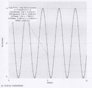
We used f(x)=Asin(Bx+C) as our function. We had x start at zero and then go to 10 by 0.1. In the equation, A = amplitude which is 5 in this equation, B = frequency which is 3, and C = phase which is pi/3.
The first picture has the equation shown. In the second picture, we have the numerical value after excel plugged in the numbers.
This is the graph of the plotted points. The x values are that of which we used in excel sheet. It starts at zero and goes to ten by 0.1. The y values are the numerical values we got after excel plugged the numbers into the equation:

The original equation is f(x)=5sin(3x+(pi/3). After doing the best fit quadratic line, out equation comes out to be f(x)=5sin(3x+1.05). This is fairly correct when pi/3 is rounded to two decimal places. We used 1.047198 for pi/3.

y(formula)=&A&2+($8$2*E:E)+(SC$2*E:E^2)
(the unclear data is input as above on this picture)

Graph # 1  ------------------> 

These are the excel spreadsheets from the second equation we did, f(x)=A+Bx+Cx^2. In this equation, A is position (x0) which equals 1000m. B is velocity (v0) which equals 50m/s. Lastly, C is gravity which equals -4.9m/s^2. For the x values, x is represented by delta t which equals 0.2. We interpreted this as the x values start at 0.2 and increase by 0.2 as well. We had it go to ten just like the last equation.

This spreadsheet "shows the equation" (bad quality) and the numerical value after excel plugged the numbers into the equation.

Graph # 2
This it the graph that comes from the second equation. The x values are delta t which starts at 0.2 and increase by 0.2. The y values are the numerical values given by plugging the numbers into the equation.
Our original equation was f(x)=1000+50x-4.9x^2. The best fit line we got was f(x)=1000+50x-4.9x^2. The equation is the exact same as the one we used.

Conclusion:

     This was a good lab exercise  because we got a chance to practice and learn how to use Microsoft EXCEL. It also helped because we were able to see how the different parts of equations affect graphs. In our group, we had initially put our acceleration (due to gravity) as positive 4.9m/s^2 instead of negative 4.9m/s^2. The only problem we had in this lab was that our graph was completely different from the one that was negative. Our parabola was upside down opening up. However, when we fixed the problem, we understood what was going on.

Vector Addition of Forces

Vector Addition of Forces

Purpose:  To study vector addition by:

1) Graphical means. 

2) Using their components by using trigonometric Calculations. 

(A circular force table is used to check our results.)

Equipment:  

• 1 Protractor
• Some String
• Various Mass Plates
• 4 Pulleys
• 1 Circular Force Table

Procedure:  (From Lab Sheet)

1.  Your instructor will give each group three masses in grams (which will
represent the magnitude of three forces) and three angles. Choose a scale of
 1 cm = 20 grams, make a vector diagram showing these forces, and
graphically find their resultant. Determine the magnitude (length) and
direction (angle) of the resultant force using a ruler and protractor. 

2. Make a second vector diagram and show the same three forces again.  Find
the resultant vector again, this time by components. Show the components of
each vector as well as the resultant vector on your diagram. Draw the force
(vector) you would need to exactly cancel out this resultant.

3. Mount three pulleys on the edge of your force table at the angles given
above. Attach strings to the center ring so that they each run over the pulley
and attach to a mass holder as shown in the figure below. Hang the
appropriate masses (numerically equal to the forces in grams) on each string.
Is the ring in equilibrium?  Set up a fourth pulley and mass holder at 180
degrees opposite from the angle you calculated for the resultant of the first
three vectors. Record all mass and angles. If you now place a mass on this
fourth holder equal to the magnitude of the resultant, what happens?  Ask
your instructor to check your results before going on.

Setup:

Our group started with magnitudes 200cm, 100cm, and 150 cm with degrees of 0, 41, and 132 respectively. This is the graph of the vectors given: 

1 cm = 20 g

     Vector D is the resultant force. The angle of vector D and the x-axis is 45 degrees.

The graph shows the x and y components of each vector as well.

Vector A) Ax = 200g                                       x = 200+100cos(41)+150cos(132) = 175.1g
                Ay = 0g                                            y = 0+100sin(41)+sin(132) = 177.1g
Vector B) Bx = 100cos(41) = 75.5g
                By = 100sin(41) = 65.6g                 R = 250g at 45 degree
Vector C) Cx = 150cos(132) = -100.4g          Rx = 250cos(45) = 176.8g
                Cy = 150sin(132) = 111.5g             Ry = 250sin(45) = 176.8g

This graph only shows the x and y components of each vector, and the resultant vector is shown going from the tail of the first to the head of the last:

1 cm = 20 g

Using

 A= angle of vector

Sin(A)= ((y component)/(magnitude of vector))

(magnitude of vector)(sin(A))=(y component)

Cos(A)= ((x component)/(magnitude of vector))

(magnitude of vector)(Cos(A))=(x component)

plugging in all of the vector data to the equation, the x-component of each vector are added to find R_x, and the y-components are also added to find R_y.

R_x=200+100cos(41)+150cos(132)

R_x=175.1

R_y=0+100sin(41)+150sin(132)

R_y=177.1

Now, using our new values of R_x=175.1 and R_y=177.1, the exact magnitude and angle of our Resultant  Vector R can be calculated.

(Magnitude of Vector R)=(175.1²+177.1²)^1/2

(Magnitude of Vector R)=249g

(Angle of Vector R)=tan^-1(177.1/175.1)

(Angle of Vector R)=45.3 degrees

The negative of Vector R then needed to be taken in order to create equilibrium between the forces. To do this, the vector components are simply transposed to negative (opposite vectors) and then take the new angle (225 degrees) is found, denoted Vector -R.

     Once the components of all the vectors had been obtained, the vectors were to be physically plotted on the circular force table. On the first holder, start with a force of 200g at 0 degrees, then add a force of 100g at an angle of 41 degrees on the second holder. Continuing,the third vector was added with mass 150g at 132 degrees on the third holder.

Question:  What happens when you place a mass on the fourth holder equal to the magnitude of the resultant vector?

     When Vector -R (which is equal in magnitude to the resultant vector, but opposite in direction) is plotted physically and placed on the fourth holder, it creates equilibrium between the forces on the circular force table.

Circular Force Table w/ all masses; Circular Force Table in Equilibrium

Top View of Circular Force Table, showing the Equilibrium created by each Vector

This is the picture from the simulation website. using our vectors, we got the same resultant vector:

Vector Check

Simulated at:

 http://phet.colorado.edu/en/simulation/vector-addition

Conclusion:
     In this lab, we were able to learn about the addition of vectors both graphically and with using components. Graphing the vectors seemed to be a reasonably accurate way to estimate the magnitude and direction, but using the vector components was able to give one a clear and precise answer to our resultant vector. Possible sources of error in this lab would include having to estimate a weight in grams to balance, or even not setting the angles precisely on the circular force table.