Working with Spreadsheets
Purpose:
To get familiar with electronic spreadsheets by using them in some simple applications.
Equipment:
- 1 Computer with Microsoft EXCEL software.
Procedure: (from lab handout)
1. Your instructor will give you a brief explanation of how a spreadsheet works and show you some
of the basic operations and functions.
2. Turn on the computer and load Excel software by clicking on Start, move the mouse over
Programs them move the mouse over Microsoft Excel and then press the left button.
3. Create a simple spreadsheet that calculates the values of the following function:
f(x) = A sin(Bx + C)
Initially choose values for of A = 5, B = 3 and C = π/3. Place these values at the right side of the
spreadsheet in the region reserved for constants. Put the words amplitude, frequency, and phase
next to each as an explanation for the meaning of each constant. Place column headings for "x"
and "f(x)" near the middle of the spreadsheet, enter a zero in the cell below "x", and enter the
formula shown above in the cell below "f(x)". Be sure to put an equal sign in front of the formula.
Create a column for values of x that run from zero to 10 radians in steps of 0.1 radians. Use the
copy feature to create these x values (Don't enter them all by hand!). Similarly, create in the next
column the corresponding values of f(x) by copying the formula shown above down through the
same number of rows (100 in all).
4. Once the generated data looks reasonable, copy this data onto the clipboard by highlighting the
contents of the two columns and choosing EDIT/COPY from the menu bar. Print out a copy of
your spreadsheet (first 20 rows or so) and also print out the spreadsheet formulas (try CTRL~). Be
sure that your rows and columns are numbered and lettered.
5. Minimize the spreadsheet window and run the Graphical Analysis program by opening the Physics
Apps icon (double click the mouse on the icon) and then double click on the Graphical Analysis
icon. Once the program loads, click on the top of the x column and then choose EDIT/PASTE to
place the data from the clipboard into your graphing program. A graph of the data should appear
in the graph window. Put appropriate labels on the horizontal and vertical axes of the graph.
6. Highlight the portion of the graph you want to analyze and choose ANALYZE/CURVE FIT from
the menu bar to direct the computer to find a function that best fits the data. From the list of
possible functions, give the computer a hint as to what type of function you expect your data to
match. The computer should display a value for A, B, and C that fit the sine curve that you are
plotting. How do these compare with the values that you started with in your spreadsheet? Make
a copy of the data and graph by selecting FILE/PRINT. Include this in your lab report.
7. Repeat the above process for a spreadsheet that calculates the position of a freely falling particle as
a function of time. This time your constants should include the acceleration of gravity, the initial
velocity, initial position, and the time increment. Start off with g = 9.8 m/s^2, v0 = 50 m/s, x0 =
1000 m and ∆t = 0.2 s. Print out the spreadsheet (calculated results and formula as in part 4).
Again copy the data into the Graphical Analysis program and obtain a graph of position vs time.
Fit this data to a function (y = A + Bx + Cx^2) which closely matches the data. Interpret the
values of A, B, and C. Get a printout of this graph with the data table. Include this printout in
your lab report.
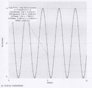
 The original equation is f(x)=5sin(3x+(pi/3). After doing the best fit quadratic line, out equation comes out to be f(x)=5sin(3x+1.05). This is fairly correct when pi/3 is rounded to two decimal places. We used 1.047198 for pi/3.
 |
| y(formula)=&A&2+($8$2*E:E)+(SC$2*E:E^2) (the unclear data is input as above on this picture) |
Graph # 1 ------------------>
These are the excel spreadsheets from the second equation we did, f(x)=A+Bx+Cx^2. In this equation, A is position (x0) which equals 1000m. B is velocity (v0) which equals 50m/s. Lastly, C is gravity which equals -4.9m/s^2. For the x values, x is represented by delta t which equals 0.2. We interpreted this as the x values start at 0.2 and increase by 0.2 as well. We had it go to ten just like the last equation.
This spreadsheet "shows the equation" (bad quality) and the numerical value after excel plugged the numbers into the equation.
Conclusion:
This was a good lab exercise because we got a chance to practice and learn how to use Microsoft EXCEL. It also helped because we were able to see how the different parts of equations affect graphs. In our group, we had initially put our acceleration (due to gravity) as positive 4.9m/s^2 instead of negative 4.9m/s^2. The only problem we had in this lab was that our graph was completely different from the one that was negative. Our parabola was upside down opening up. However, when we fixed the problem, we understood what was going on.


No comments:
Post a Comment