Working with Spreadsheets

Purpose:

To get familiar with electronic spreadsheets by using them in some simple applications.

Equipment:

• 1 Computer with Microsoft EXCEL software.

Procedure: (from lab handout)

1. Your instructor will give you a brief explanation of how a spreadsheet works and show you some 

of the basic operations and functions. 

2. Turn on the computer and load Excel software by clicking on Start, move the mouse over              

Programs them move the mouse over Microsoft Excel and then press the left button. 

3. Create a simple spreadsheet that calculates the values of the following function: 

    f(x) = A sin(Bx + C) 

   

Initially choose values for  of  A = 5, B = 3 and  C = π/3.  Place these values at the right side of the 

spreadsheet in the region reserved for constants.  Put the words amplitude, frequency, and phase 

next to each as an explanation for the meaning of each constant.  Place column headings for "x" 

and "f(x)" near the middle of the spreadsheet, enter a zero in the cell below "x", and enter the 

formula shown above in the cell below "f(x)".  Be sure to put an equal sign in front of the formula.  

Create a column for values of x that run from zero to 10 radians in steps of  0.1 radians.  Use the 

copy feature to create these x values (Don't enter them all by hand!).  Similarly, create in the next 

column the corresponding values of  f(x) by copying the formula shown above down through the 

same number of rows (100 in all). 

4. Once the generated data looks reasonable, copy this data onto the clipboard  by highlighting the 

contents of the two columns and choosing  EDIT/COPY from the menu bar. Print out a copy of 

your spreadsheet (first 20 rows or so) and also print out the spreadsheet formulas (try CTRL~).  Be 

sure that your rows and columns are numbered and lettered. 

5. Minimize the spreadsheet window and run the Graphical Analysis program by opening the Physics 

Apps icon (double click the mouse on the icon) and then double click on the Graphical Analysis

icon.  Once the program loads, click on the top of the x column and then choose EDIT/PASTE to 

place the data from the clipboard into your graphing program.  A graph of the data should appear 

in the graph window.  Put appropriate labels on the horizontal and vertical axes of the graph.  

6. Highlight the portion of the graph you want to analyze and choose ANALYZE/CURVE FIT from 

the menu bar to direct the computer to find a function that best fits the data.  From the list of 

possible functions, give the computer a hint as to what type of function you expect your data to 

match.  The computer should display a value for A, B, and C that fit the sine curve that you are 

plotting.  How do these compare with the values that you started with in your spreadsheet?  Make 

a copy of the data and graph by selecting FILE/PRINT.  Include this in your lab report. 

7. Repeat the above process for a spreadsheet that calculates the position of a freely falling particle as 

a function of time.  This time your constants should include the acceleration of gravity, the initial 

velocity, initial position, and the time increment.  Start off with g = 9.8 m/s^2, v0 = 50 m/s, x0 = 

1000 m and ∆t = 0.2 s.  Print out the spreadsheet (calculated results and formula as in part 4).  

Again copy the data into the Graphical Analysis program and obtain a graph of position vs time.  

Fit this data to a function  (y = A + Bx + Cx^2) which closely matches the data.  Interpret the 

values of  A, B, and C.  Get a printout of this graph with the data table.  Include this printout in 

your lab report.

  

1st Spreadsheet

We used f(x)=Asin(Bx+C) as our function. We had x start at zero and then go to 10 by 0.1. In the equation, A = amplitude which is 5 in this equation, B = frequency which is 3, and C = phase which is pi/3.
The first picture has the equation shown. In the second picture, we have the numerical value after excel plugged in the numbers.
This is the graph of the plotted points. The x values are that of which we used in excel sheet. It starts at zero and goes to ten by 0.1. The y values are the numerical values we got after excel plugged the numbers into the equation:

The original equation is f(x)=5sin(3x+(pi/3). After doing the best fit quadratic line, out equation comes out to be f(x)=5sin(3x+1.05). This is fairly correct when pi/3 is rounded to two decimal places. We used 1.047198 for pi/3.

y(formula)=&A&2+($8$2*E:E)+(SC$2*E:E^2)
(the unclear data is input as above on this picture)

Graph # 1  ------------------> 

These are the excel spreadsheets from the second equation we did, f(x)=A+Bx+Cx^2. In this equation, A is position (x0) which equals 1000m. B is velocity (v0) which equals 50m/s. Lastly, C is gravity which equals -4.9m/s^2. For the x values, x is represented by delta t which equals 0.2. We interpreted this as the x values start at 0.2 and increase by 0.2 as well. We had it go to ten just like the last equation.

This spreadsheet "shows the equation" (bad quality) and the numerical value after excel plugged the numbers into the equation.

Graph # 2
This it the graph that comes from the second equation. The x values are delta t which starts at 0.2 and increase by 0.2. The y values are the numerical values given by plugging the numbers into the equation.
Our original equation was f(x)=1000+50x-4.9x^2. The best fit line we got was f(x)=1000+50x-4.9x^2. The equation is the exact same as the one we used.

Conclusion:

     This was a good lab exercise  because we got a chance to practice and learn how to use Microsoft EXCEL. It also helped because we were able to see how the different parts of equations affect graphs. In our group, we had initially put our acceleration (due to gravity) as positive 4.9m/s^2 instead of negative 4.9m/s^2. The only problem we had in this lab was that our graph was completely different from the one that was negative. Our parabola was upside down opening up. However, when we fixed the problem, we understood what was going on.

Vector Addition of Forces

Vector Addition of Forces

Purpose:  To study vector addition by:

1) Graphical means. 

2) Using their components by using trigonometric Calculations. 

(A circular force table is used to check our results.)

Equipment:  

• 1 Protractor
• Some String
• Various Mass Plates
• 4 Pulleys
• 1 Circular Force Table

Procedure:  (From Lab Sheet)

1.  Your instructor will give each group three masses in grams (which will
represent the magnitude of three forces) and three angles. Choose a scale of
 1 cm = 20 grams, make a vector diagram showing these forces, and
graphically find their resultant. Determine the magnitude (length) and
direction (angle) of the resultant force using a ruler and protractor. 

2. Make a second vector diagram and show the same three forces again.  Find
the resultant vector again, this time by components. Show the components of
each vector as well as the resultant vector on your diagram. Draw the force
(vector) you would need to exactly cancel out this resultant.

3. Mount three pulleys on the edge of your force table at the angles given
above. Attach strings to the center ring so that they each run over the pulley
and attach to a mass holder as shown in the figure below. Hang the
appropriate masses (numerically equal to the forces in grams) on each string.
Is the ring in equilibrium?  Set up a fourth pulley and mass holder at 180
degrees opposite from the angle you calculated for the resultant of the first
three vectors. Record all mass and angles. If you now place a mass on this
fourth holder equal to the magnitude of the resultant, what happens?  Ask
your instructor to check your results before going on.

Setup:

Our group started with magnitudes 200cm, 100cm, and 150 cm with degrees of 0, 41, and 132 respectively. This is the graph of the vectors given: 

1 cm = 20 g

     Vector D is the resultant force. The angle of vector D and the x-axis is 45 degrees.

The graph shows the x and y components of each vector as well.

Vector A) Ax = 200g                                       x = 200+100cos(41)+150cos(132) = 175.1g
                Ay = 0g                                            y = 0+100sin(41)+sin(132) = 177.1g
Vector B) Bx = 100cos(41) = 75.5g
                By = 100sin(41) = 65.6g                 R = 250g at 45 degree
Vector C) Cx = 150cos(132) = -100.4g          Rx = 250cos(45) = 176.8g
                Cy = 150sin(132) = 111.5g             Ry = 250sin(45) = 176.8g

This graph only shows the x and y components of each vector, and the resultant vector is shown going from the tail of the first to the head of the last:

1 cm = 20 g

Using

 A= angle of vector

Sin(A)= ((y component)/(magnitude of vector))

(magnitude of vector)(sin(A))=(y component)

Cos(A)= ((x component)/(magnitude of vector))

(magnitude of vector)(Cos(A))=(x component)

plugging in all of the vector data to the equation, the x-component of each vector are added to find R_x, and the y-components are also added to find R_y.

R_x=200+100cos(41)+150cos(132)

R_x=175.1

R_y=0+100sin(41)+150sin(132)

R_y=177.1

Now, using our new values of R_x=175.1 and R_y=177.1, the exact magnitude and angle of our Resultant  Vector R can be calculated.

(Magnitude of Vector R)=(175.1²+177.1²)^1/2

(Magnitude of Vector R)=249g

(Angle of Vector R)=tan^-1(177.1/175.1)

(Angle of Vector R)=45.3 degrees

The negative of Vector R then needed to be taken in order to create equilibrium between the forces. To do this, the vector components are simply transposed to negative (opposite vectors) and then take the new angle (225 degrees) is found, denoted Vector -R.

     Once the components of all the vectors had been obtained, the vectors were to be physically plotted on the circular force table. On the first holder, start with a force of 200g at 0 degrees, then add a force of 100g at an angle of 41 degrees on the second holder. Continuing,the third vector was added with mass 150g at 132 degrees on the third holder.

Question:  What happens when you place a mass on the fourth holder equal to the magnitude of the resultant vector?

     When Vector -R (which is equal in magnitude to the resultant vector, but opposite in direction) is plotted physically and placed on the fourth holder, it creates equilibrium between the forces on the circular force table.

Circular Force Table w/ all masses; Circular Force Table in Equilibrium

Top View of Circular Force Table, showing the Equilibrium created by each Vector

This is the picture from the simulation website. using our vectors, we got the same resultant vector:

Vector Check

Simulated at:

 http://phet.colorado.edu/en/simulation/vector-addition

Conclusion:
     In this lab, we were able to learn about the addition of vectors both graphically and with using components. Graphing the vectors seemed to be a reasonably accurate way to estimate the magnitude and direction, but using the vector components was able to give one a clear and precise answer to our resultant vector. Possible sources of error in this lab would include having to estimate a weight in grams to balance, or even not setting the angles precisely on the circular force table.

Acceleration of Gravity on an Inclined Plane 

Purpose:

1.  To find the acceleration of gravity by studying the motion of a cart on an incline.
2.  To gain further experience using the computer for data collection and analysis. 

Equipment Needed:

• 1 windows based computer with Logger Pro software
• 1 motion detector
• 1 ballistic cart
• aluminum track
• 1 wood blocks
• 1 meter stick
• 1 small carpenter level  

Introduction:
     In this laboratory you will use the computer to collect position (x) vs time (t) data for a cart accelerating on an inclined track.  By comparing the acceleration of  the cart when moving up and down the track, the effect of friction can be eliminated and the acceleration due to the effect of gravity alone can be found.  Since the force of friction acts with the force of gravity when the cart is going up the track and against the force of gravity when the cart is going down the track, we can average the slightly increased acceleration (when going up) with the slightly decreased acceleration (when going down) to obtain an acceleration that depends only on the force of gravity.  If we call g the acceleration due to gravity when an object is in free fall, then the component of this acceleration along the track is g sinθ where θ is the angle of incline for the track.Because the force of friction acts with the motion of the cart on the way up ramp, and acts against the motion on the way down the ramp, the average of the two accelerations will be taken with the following ratio:

gsin(A)= (a₁+a₂)/2

where g= gravity, A= angle of incline, a₁= acceleration up incline, and a₂= acceleration down incline.

In this lab we will measure acceleration by looking at the slope of the v vs t curve for the cart.

Procedure:
(from lab)

1. Connect labpro to computer and motion detector to DIG/SONIC2 port on labpro. Turn on the computer and load the logger pro software.  Set up the logger pro software by opening the "graphlab" file in the mechanics folder.
2. Set up the Track and slightly increase the incline by putting a wooden block under it. Make sure the track is leveled. Once you have done this, Determine the inclination angle by using the method on FIGURE #1.
3. Place the motion detector at the upper end of the track facing the lower end.  The Ballistic cart should start at the lower end of the track.  Now gently push the cart towards the motion detector.  Make sure the cart does not reach 50 cm close to the motion detector ( it will prevent motion detector from detecting it).
4. Start the data collector a few seconds before you push the cart. As the cart leaves your hand watch the v vs t graph and the x vs t. The v vs t graph should form a parabolic section. If  not repeat the process
5. Once the Graphs are complete. You should now figure out the Acceleration using both graphs. For the Position vs time graph, Use the "CURVE FIT" option in the logger pro program.  For the Velocity vs time graph, use the Linear fit instead. Now use trig to find the y component of the acceleration vector, label acceleration as a1 in x vs t, and a2 for v vs t. 
6. Repeat steps 4 and 5 two more times with the same incline. (the Average of the values should be close to 9.8 m/s^2)
7. Repeat the Experiment with a different incline.

We set up the aluminum track at an incline with the wooden block, and then carefully leveled it out. Then, we measured the change in height of the two sides, to the horizontal length of the inclined ramp. The Calculations of the ramp's angle are as followed: 

Tan^-1((y₂-y₁)/(x₂-x₁))=A

Tan^-1((12.9cm-6.7cm)/(228.2cm))=A

A=1.56^o

The Set-up for our Experiment

Once we set up, three trial runs were completed first for the incline at the angle of 1.56 degrees, and then we conducted three trails for incline set to an angle of 3.6 degrees.

*Question: What type of curve will we expect to see for the x vs. t graphs and v vs. t graphs? 

     We expected that the graph of x vs. t would be a parabolic with the left side having a more drastic change in slope than the right side, since friction will be acting with the motion of the cart on the way up and against it on the way down. We also expected the graph of v vs. t to be linear with different slopes for the motion up and the motion down the ramp, since friction would affect the acceleration of the cart.

Results:

Position vs. Time Graph

Velocity vs. Time Graph w/ Line of Best Fit

A linear fit was applied to the negative velocity portion of the v vs. t graph for a₁, as well as a linear fit to the positive velocity of the v vs. t graph for a₂ in order to get values for a₁ and a₂.

Since the derivative of velocity is acceleration, we used the slopes of our best fit lines in order to obtain out accelerations.

The following is our data for each of the trial runs:

Conclusion:

Once the data had been collected, verification of our numbers compared to the accepted value of acceleration due to gravity was needed. Since the force of friction acts with the force of gravity on the way up the ramp and against it on the way down, the average of the two accelerations will be taken to equate our experimental value of acceleration due to gravity. The formula used to calculate G_exp was:

G_expsin(1.56)=(a₁+a₂)/2

-Trial one of 1.56 degree incline

G_expsin(1.56)=(0.33 m/s²+0.18 m/s²)/2

G_exp=9.4m/s²

In this lab we were able to determine the effect gravity has on objects that are on inclined planes pretty accurately. The percentage differences we calculated in this lab seemed to match well with the accepted 9.8 m/s². Our most inconsistent value was 9.4 m/s² with a 4.1% difference. Potential sources of error in this lab could have included various factors such as the friction between the car and the track, and performing the linear fit to the velocity vs. time graphs in different domains. 

Acceleration of Gravity Lab

Acceleration of Gravity Lab

Lab Partners :  Kevin Hilario, Becca Causey, and Raychel Kolofske

Purpose : 

To determine the acceleration of gravity for a freely falling object, and to gain experience using the computer as a data collector. (We have to be able to determine the acceleration due to gravity by observing an object in free fall, and practice recording data using the computer's data collector.)

Equipment Needed :

• 1 Windows based computer with the Logger Pro software

• 1 Lab Pro interface

• 1 motion detector

• 1 rubber ball

• 1 wire basket

 Procedure :

1.  Connect the lab pro to computer and motion detector to DIG/SONIC2 port on lab pro. Turn on the

computer and load the Logger Pro software by double clicking on its icon located within the Physics

Apps folder. A file named graphlab will be used to set up the computer for collecting the data needed

for this experiment.  To open this file, first select File/Open and then open the mechanics folder. 

When this folder opens, open the graphlab file.

2.  You should see a blank position vs. time graph.  The vertical scale (position axis) should be from 0 to 4m while the horizontal scale (time axis) should be from 0 to 4 s.  These values can be changed if you desire by pointing the mouse at the upper and lower limits on either scale and clicking on the number to be changed.  Enter in the desired numbers and push the Enter key.

3.  Place the motion detector on the floor facing upward and place the wire basket (inverted) over the detector for protection from the falling ball.  Check to see that the motion detector is working properly by holding the rubber ball about 1 m above the detector.  Have your lab partner click on Collect button to begin taking data and then move your hand up and down a few times and verify that the graph of the motion is consistent with the actual motion of your hand.  After 4s the computer will stop taking data and will be ready for another trial.  If your equipment does not seem to be working properly ask for help.

4.  Give the ball a gentle toss straight up from a point about 1 meter above the detector.  The ball should rise 1 or 2 m above where your hand released the ball.  Ideally your toss should result in the ball going straight up and down directly above the detector.  It will take a few tries to perfect your toss.  Be

aware of what your hands are doing after the toss as they may interfere with the path of the ultrasonic

waves as they travel from the detector to the ball and back.  Take your time and practice until you can

get a position-time graph that has a nice parabolic shape.  Why should it be a parabola?

5. Select the data in the interval that corresponds to the ball in free-fall by clicking and dragging the mouse across the parabolic portion of the graph.  Release the mouse button at the end of this data range.  Any later data analysis done by the program will use only the data from this range.  Choose Analyze/Curve Fit from the menu at the top of the window.  Choose a t^2+ b t + c (Quadratic) and let the computer find the values of a, b, and c that best fit the data.  If the fitted curve matches the data curve, select Try Fit.  Click on OK if the fit looks good.  A box should appear on the graph that contains the values of a, b, and c.  Give a physical interpretation and the proper units for each of these quantities (Hint: use unit analysis).  Find the acceleration, g-exp, of the ball from this data and calculate the percent difference between this value and the accepted value, g-acc, (9.80 m/s^2).

  

6. Look at a graph of velocity vs time for this motion by double clicking on the y-axis label and select

“velocity” and deselect “position”.  Examine this graph carefully.  Explain (relate them to the actual

motion of the ball) the regions where the velocity is negative, positive, and where it reaches zero.  Why

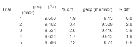
does the curve have a negative slope?  What does the slope of this graph represent?  Determine the slope from a linear curve fit to the data.  Find the values of m and b that best fit the data. Give a physical interpretation and the proper units for each of these quantities (Hint: use unit analysis). Find the acceleration of the ball, g-exp,  from this data and calculate the percent difference between this value and the accepted value, g-acc.  Put together an excel spreadsheet for your data like the one shown below. Finally, select Experiment/Store Latest Run to prepare for the next trial.

7.  Repeat steps 4 - 6 for at least five more trials.  Obtain an average value for the acceleration of gravity and a percent difference between this value and the accepted value.

8.  Obtain a printout of one representative graph for position vs time and velocity vs. time and include this in your lab report.  Put both graphs on a single page.

Results:

Position vs Time Graph w/ best fit Parabola

Velocity vs Time Graph w/ best fit Line

%Difference Spreadsheet for 5 Trails

Motion Diagram for Position vs Time

We labeled the origin and the positive direction. Also, we showed the direction of acceleration. Where the purple arrow is, it shouldn't say a=0, but say v=0 instead. On the left side it shows that the ball is decreasing in motion in the positive direction. On the right side, the ball is moving in the negative direction and is increasing. The point where there is a break in the motion diagram, connected by the pink, dashed,curved line, is where v=0 because there is the point where the ball begins to descend.

Conclusion:

In this lab we found the velocity and acceleration from the path of a ball being tossed in the air. With those we found the difference in what we found and what is actual. Nothing was perfect, because a ball thrown by a person can not be a perfect parabola. That is why we did more than one trial so that we can  get as close to perfect as possible. For all of the velocity, the differences were less than four percent. However, over all the difference for acceleration beat velocity except for one trial. Trials 2-5 were all less than four percent as well. The first trial was less than seven percent. Trial five for acceleration was less than one percent leaving it to be the best over all.