Acceleration of Gravity on an Inclined Plane 

Purpose:

1.  To find the acceleration of gravity by studying the motion of a cart on an incline.
2.  To gain further experience using the computer for data collection and analysis. 

Equipment Needed:

• 1 windows based computer with Logger Pro software
• 1 motion detector
• 1 ballistic cart
• aluminum track
• 1 wood blocks
• 1 meter stick
• 1 small carpenter level  

Introduction:
     In this laboratory you will use the computer to collect position (x) vs time (t) data for a cart accelerating on an inclined track.  By comparing the acceleration of  the cart when moving up and down the track, the effect of friction can be eliminated and the acceleration due to the effect of gravity alone can be found.  Since the force of friction acts with the force of gravity when the cart is going up the track and against the force of gravity when the cart is going down the track, we can average the slightly increased acceleration (when going up) with the slightly decreased acceleration (when going down) to obtain an acceleration that depends only on the force of gravity.  If we call g the acceleration due to gravity when an object is in free fall, then the component of this acceleration along the track is g sinθ where θ is the angle of incline for the track.Because the force of friction acts with the motion of the cart on the way up ramp, and acts against the motion on the way down the ramp, the average of the two accelerations will be taken with the following ratio:

gsin(A)= (a₁+a₂)/2

where g= gravity, A= angle of incline, a₁= acceleration up incline, and a₂= acceleration down incline.

In this lab we will measure acceleration by looking at the slope of the v vs t curve for the cart.

Procedure:
(from lab)

1. Connect labpro to computer and motion detector to DIG/SONIC2 port on labpro. Turn on the computer and load the logger pro software.  Set up the logger pro software by opening the "graphlab" file in the mechanics folder.
2. Set up the Track and slightly increase the incline by putting a wooden block under it. Make sure the track is leveled. Once you have done this, Determine the inclination angle by using the method on FIGURE #1.
3. Place the motion detector at the upper end of the track facing the lower end.  The Ballistic cart should start at the lower end of the track.  Now gently push the cart towards the motion detector.  Make sure the cart does not reach 50 cm close to the motion detector ( it will prevent motion detector from detecting it).
4. Start the data collector a few seconds before you push the cart. As the cart leaves your hand watch the v vs t graph and the x vs t. The v vs t graph should form a parabolic section. If  not repeat the process
5. Once the Graphs are complete. You should now figure out the Acceleration using both graphs. For the Position vs time graph, Use the "CURVE FIT" option in the logger pro program.  For the Velocity vs time graph, use the Linear fit instead. Now use trig to find the y component of the acceleration vector, label acceleration as a1 in x vs t, and a2 for v vs t. 
6. Repeat steps 4 and 5 two more times with the same incline. (the Average of the values should be close to 9.8 m/s^2)
7. Repeat the Experiment with a different incline.

We set up the aluminum track at an incline with the wooden block, and then carefully leveled it out. Then, we measured the change in height of the two sides, to the horizontal length of the inclined ramp. The Calculations of the ramp's angle are as followed: 

Tan^-1((y₂-y₁)/(x₂-x₁))=A

Tan^-1((12.9cm-6.7cm)/(228.2cm))=A

A=1.56^o

The Set-up for our Experiment

Once we set up, three trial runs were completed first for the incline at the angle of 1.56 degrees, and then we conducted three trails for incline set to an angle of 3.6 degrees.

*Question: What type of curve will we expect to see for the x vs. t graphs and v vs. t graphs? 

     We expected that the graph of x vs. t would be a parabolic with the left side having a more drastic change in slope than the right side, since friction will be acting with the motion of the cart on the way up and against it on the way down. We also expected the graph of v vs. t to be linear with different slopes for the motion up and the motion down the ramp, since friction would affect the acceleration of the cart.

Results:

Position vs. Time Graph

Velocity vs. Time Graph w/ Line of Best Fit

A linear fit was applied to the negative velocity portion of the v vs. t graph for a₁, as well as a linear fit to the positive velocity of the v vs. t graph for a₂ in order to get values for a₁ and a₂.

Since the derivative of velocity is acceleration, we used the slopes of our best fit lines in order to obtain out accelerations.

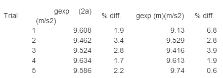
The following is our data for each of the trial runs:

Conclusion:

Once the data had been collected, verification of our numbers compared to the accepted value of acceleration due to gravity was needed. Since the force of friction acts with the force of gravity on the way up the ramp and against it on the way down, the average of the two accelerations will be taken to equate our experimental value of acceleration due to gravity. The formula used to calculate G_exp was:

G_expsin(1.56)=(a₁+a₂)/2

-Trial one of 1.56 degree incline

G_expsin(1.56)=(0.33 m/s²+0.18 m/s²)/2

G_exp=9.4m/s²

In this lab we were able to determine the effect gravity has on objects that are on inclined planes pretty accurately. The percentage differences we calculated in this lab seemed to match well with the accepted 9.8 m/s². Our most inconsistent value was 9.4 m/s² with a 4.1% difference. Potential sources of error in this lab could have included various factors such as the friction between the car and the track, and performing the linear fit to the velocity vs. time graphs in different domains. 

Acceleration of Gravity Lab

Acceleration of Gravity Lab

Lab Partners :  Kevin Hilario, Becca Causey, and Raychel Kolofske

Purpose : 

To determine the acceleration of gravity for a freely falling object, and to gain experience using the computer as a data collector. (We have to be able to determine the acceleration due to gravity by observing an object in free fall, and practice recording data using the computer's data collector.)

Equipment Needed :

• 1 Windows based computer with the Logger Pro software

• 1 Lab Pro interface

• 1 motion detector

• 1 rubber ball

• 1 wire basket

 Procedure :

1.  Connect the lab pro to computer and motion detector to DIG/SONIC2 port on lab pro. Turn on the

computer and load the Logger Pro software by double clicking on its icon located within the Physics

Apps folder. A file named graphlab will be used to set up the computer for collecting the data needed

for this experiment.  To open this file, first select File/Open and then open the mechanics folder. 

When this folder opens, open the graphlab file.

2.  You should see a blank position vs. time graph.  The vertical scale (position axis) should be from 0 to 4m while the horizontal scale (time axis) should be from 0 to 4 s.  These values can be changed if you desire by pointing the mouse at the upper and lower limits on either scale and clicking on the number to be changed.  Enter in the desired numbers and push the Enter key.

3.  Place the motion detector on the floor facing upward and place the wire basket (inverted) over the detector for protection from the falling ball.  Check to see that the motion detector is working properly by holding the rubber ball about 1 m above the detector.  Have your lab partner click on Collect button to begin taking data and then move your hand up and down a few times and verify that the graph of the motion is consistent with the actual motion of your hand.  After 4s the computer will stop taking data and will be ready for another trial.  If your equipment does not seem to be working properly ask for help.

4.  Give the ball a gentle toss straight up from a point about 1 meter above the detector.  The ball should rise 1 or 2 m above where your hand released the ball.  Ideally your toss should result in the ball going straight up and down directly above the detector.  It will take a few tries to perfect your toss.  Be

aware of what your hands are doing after the toss as they may interfere with the path of the ultrasonic

waves as they travel from the detector to the ball and back.  Take your time and practice until you can

get a position-time graph that has a nice parabolic shape.  Why should it be a parabola?

5. Select the data in the interval that corresponds to the ball in free-fall by clicking and dragging the mouse across the parabolic portion of the graph.  Release the mouse button at the end of this data range.  Any later data analysis done by the program will use only the data from this range.  Choose Analyze/Curve Fit from the menu at the top of the window.  Choose a t^2+ b t + c (Quadratic) and let the computer find the values of a, b, and c that best fit the data.  If the fitted curve matches the data curve, select Try Fit.  Click on OK if the fit looks good.  A box should appear on the graph that contains the values of a, b, and c.  Give a physical interpretation and the proper units for each of these quantities (Hint: use unit analysis).  Find the acceleration, g-exp, of the ball from this data and calculate the percent difference between this value and the accepted value, g-acc, (9.80 m/s^2).

  

6. Look at a graph of velocity vs time for this motion by double clicking on the y-axis label and select

“velocity” and deselect “position”.  Examine this graph carefully.  Explain (relate them to the actual

motion of the ball) the regions where the velocity is negative, positive, and where it reaches zero.  Why

does the curve have a negative slope?  What does the slope of this graph represent?  Determine the slope from a linear curve fit to the data.  Find the values of m and b that best fit the data. Give a physical interpretation and the proper units for each of these quantities (Hint: use unit analysis). Find the acceleration of the ball, g-exp,  from this data and calculate the percent difference between this value and the accepted value, g-acc.  Put together an excel spreadsheet for your data like the one shown below. Finally, select Experiment/Store Latest Run to prepare for the next trial.

7.  Repeat steps 4 - 6 for at least five more trials.  Obtain an average value for the acceleration of gravity and a percent difference between this value and the accepted value.

8.  Obtain a printout of one representative graph for position vs time and velocity vs. time and include this in your lab report.  Put both graphs on a single page.

Results:

Position vs Time Graph w/ best fit Parabola

Velocity vs Time Graph w/ best fit Line

%Difference Spreadsheet for 5 Trails

Motion Diagram for Position vs Time

We labeled the origin and the positive direction. Also, we showed the direction of acceleration. Where the purple arrow is, it shouldn't say a=0, but say v=0 instead. On the left side it shows that the ball is decreasing in motion in the positive direction. On the right side, the ball is moving in the negative direction and is increasing. The point where there is a break in the motion diagram, connected by the pink, dashed,curved line, is where v=0 because there is the point where the ball begins to descend.

Conclusion:

In this lab we found the velocity and acceleration from the path of a ball being tossed in the air. With those we found the difference in what we found and what is actual. Nothing was perfect, because a ball thrown by a person can not be a perfect parabola. That is why we did more than one trial so that we can  get as close to perfect as possible. For all of the velocity, the differences were less than four percent. However, over all the difference for acceleration beat velocity except for one trial. Trials 2-5 were all less than four percent as well. The first trial was less than seven percent. Trial five for acceleration was less than one percent leaving it to be the best over all.

Graphical Analysis Lab

Graphical Analysis Lab

Lab Partner: Keith Sylvester

Purpose:  To gain experience in drawing graphs and in using graphing software.
(We basically learned how to use and became familiar with using the Graphical Analysis software.)

Equipment Needed :

• 1 Windows based computer with the Graphical Analysis and the Logger Pro software
• 1 Lab Pro interface
• 1 motion detector
• 1 rubber ball
• 1 wire basket

Procedure:

PART I

     First we had to log onto the computer provided for us and locate the Graphical Analysis software in the appropriate folder.  We then proceeded to find and open a designated, pre-existing file that was saved onto the computer.  The file had the tables of data and a generic graph.  We then had to chose one of the sets of data (X2) and manipulate the graph by changing the formula from the form F(x) = x, where x = X2 = the second set of data, to whatever formula we chose to manipulate the graph with.  We chose to change the function from F(x) = x, to F(x) = sin(x)\x.  We then had to crop and label the graph.  The results of the change can be seen in the graphs below:

(print out of how the graph looks on the software)

(a colorful version that we shared in class)

PART II

     For the second part of the lab we had to log into another software called Logger Pro.  After connecting the Lab Pro interface to the computer, and the motion detector to the Lab Pro hardware, we set the motion detector on the floor and covered it by putting the wire basket upside down over it.  We then practiced detecting the motion of a falling ball by starting collecting the data on Logger Pro and dropping the ball onto the wire basket, just above the motion detector.  Once we became comfortable doing this, we did one last trail and obtained the graph of the motion of a falling ball, which can be seen below:



(the darker line represents our best fit parabola and the zig-zag lines represent the ball bouncing in and out of the range of the motion detector)

(This the graph that we shared with the class which includes the equation for our best fit parabola,
x =  -4.475t^2+1.055t+1.477, and our axis and unit labels  where time was our x-axis with units in seconds, and our y-axis is position with its units being meters.)

* A question asks: d α gt^n where g = 9.8 m/s^2, is the acceleration due to gravity.  What is n in this equation?

*The n is the highest power of out equation, which n = 2 in this instance, and  what type of equation the graph is, which is parabolic(quadratic) in our case.

You can see the relationship between Unit Analysis and Dimensional Analysis by using Algebra. You can prove your Dimensional Analysis through Unit Analysis by showing that both sides of the equation end up with the same units.

Dimensional Analysis : t = (d / g)^(1/2)~~time = (distance / acceleration due to gravity)^(1/2) ~~~ time is equal to the square root of the distance divided by the acceleration due to gravity.

Unit Analysis :  s = (m / (m/s^2))^(1/2) ---mass cancelled out---> s = (1/(1/s^2))^(1/2)---1/(1/s^2) is equal to s^2---> s = (s^2)^(1/2) ---squaring and square root cancelled out---> ∴ s = s

Conclusion : I was slightly familiar with the Logger Pro from taking Chem-1A, but I haven't used it in for about two semesters, so, for me, this lab was a nice review on how the system works.  I now feel comfortable using both the Graphical Analysis software and the logger Pro software.